Simulate neural dynamics using a wave model

In this tutorial we will use the geometric eigenmodes and eigenvalues to simulate cortical activity, using the Pang et al. (2023) model based on neural field theory. Here, the spatiotemporal evolution of activity \(\phi(\vec r,t)\) is described by an isotropic damped wave equation without regeneration,

\[ \displaystyle \bigg[\frac{1}{\gamma_s^2}\frac{\partial^2}{\partial t^2} +\frac{2}{\gamma_s}\frac{\partial}{\partial t}+1-r_s^2\nabla^2 \bigg]\phi(\vec r,t)=Q(\vec r,t), \]

where:

• \(\gamma_s\) denotes the temporal damping parameter

• \(r_s\) denotes the spatial length scale parameter

• \(\nabla^2\) denotes the Laplace-Beltrami operator

• \(Q(\vec r,t)\) denotes external input

As in the previous tutorials, we begin by initialising the EigenSolver with a cortical surface and medial wall mask, then solve for the first 200 eigenmodes. This time we can try out the macaque data.

from neuromodes.io import fetch_surf
from neuromodes import EigenSolver
from nsbutils.utils import unmask
from nsbutils.plotting import plot_surf
from importlib.resources import files, as_file

mesh, medmask = fetch_surf(species='macaque')
solver = EigenSolver(mesh, mask=medmask).solve(200)

We can then call the simulate_waves class method to compute timeseries of neural activity:

sim_ts = solver.simulate_waves()

Note that 1000 timepoints (nt) are simulated by default, with a timestep of \(10^{-4}\) seconds (dt), using Gaussian white noise as external input.

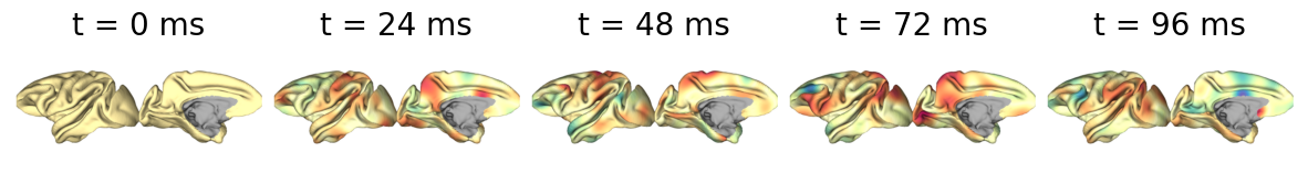
To visualise activity, we can first sample a few timepoints from the output and add the medial wall back in by using unmask from nsbutils:

sim_ts_sample = unmask(sim_ts[:, ::240], medmask)  # Sample every 240 time points

Each of these sampled timepoints can be visualised with plot_surf from nsbutils:

lh_surfpath = files('neuromodes.data') / 'sp-macaque_tpl-fsLR_den-32k_hemi-L_midthickness.surf.gii'
with as_file(lh_surfpath) as lh_surfpath: 
    plot_surf(
        lh_surfpath,
        sim_ts_sample,
        labels=[f't = {i*24} ms' for i in range(5)],
        cmap='Spectral',
        color_range='group'
    )