Model a structural connectome

This tutorial will demonstrate how to generate a structural connectivity matrix \(G\) using the Normand et al. (2025) model,

\[ \displaystyle G_{ij}=\sum_{m=1}^k \frac{\psi_m(i)\psi_m^+(j)}{1+r_s^2\lambda_m}, \]

where:

• \(G_{ij}\) denotes the connectivity strength between cortical vertices \(i\) and \(j\)

• \(\psi_m(i)\) denotes the amplitude of the \(m^{th}\) geometric eigenmode at vertex \(i\)

• \(\lambda_m\) denotes the \(m^{th}\) eigenvalue

• \([\ \ ]^+\) denotes the Moore–Penrose pseudoinverse

• \(r_s\) denotes the spatial length scale parameter

• \(k\) denotes the number of modes used

As in the previous tutorials, we begin by initialising the EigenSolver with a cortical surface and medial wall mask, then solving for the first 120 eigenmodes. To reduce computation and plotting time, we can use the fsLR-4k mesh.

from importlib.resources import files, as_file
from neuromodes import EigenSolver
from neuromodes.io import fetch_surf
from nsbutils.plotting import plot_surf, plot_heatmap
from nsbutils.utils import unmask

mesh, medmask = fetch_surf(density='4k', hemi='R')
solver = EigenSolver(mesh, mask=medmask).solve(120)

We can then call the model_connectome class method:

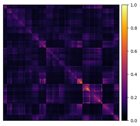
G = solver.model_connectome()

Note that \(r_s=9.53\) and \(k=108\) are used by default, in line with the paper.

We can visualise the structural connectivity matrix using plot_heatmap, from our nsbutils package:

plot_heatmap(G, cmap='inferno', cbar=True)

<Axes: >

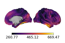
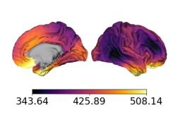
We can also visualise the vertex-averaged connectivity on the cortical surface, this time using plot_surf from nsbutils:

nodal_sc = G.sum(axis=0)

# Path to surface
rh_surfpath = files('neuromodes.data') / 'sp-human_tpl-fsLR_den-4k_hemi-R_midthickness.surf.gii'

with as_file(rh_surfpath) as rh_surfpath: 
    plot_surf(
        rh_surfpath,
        unmask(nodal_sc, medmask),
        cmap='inferno',
        cbar=True
    )

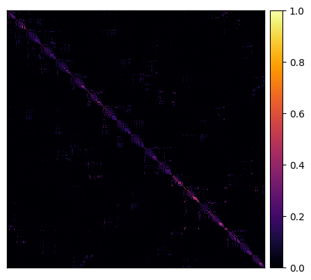
To explore the model further, we can generate another connectome but only use 5 modes instead of the default 108:

G_k5 = solver.model_connectome(k=5)

plot_heatmap(G_k5, cmap='inferno', cbar=True)

with as_file(rh_surfpath) as rh_surfpath: 
    plot_surf(
        rh_surfpath,
        unmask(G_k5.sum(axis=0), medmask),
        cmap='inferno',
        cbar=True
    )

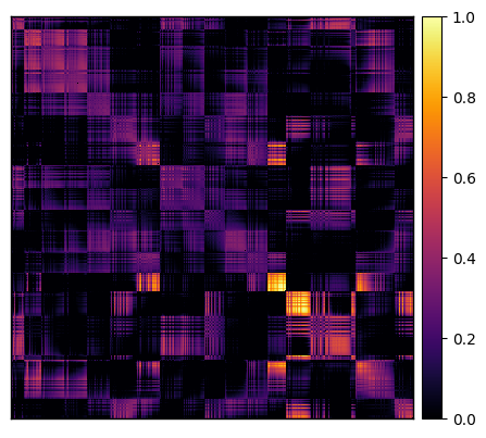
What about if we instead increase the spatial length scale parameter from 9.53 to 95.3?

G_r95 = solver.model_connectome(r=95.3)

plot_heatmap(G_r95, cmap='inferno', cbar=True)

with as_file(rh_surfpath) as rh_surfpath: 
    plot_surf(
        rh_surfpath,
        unmask(G_r95.sum(axis=0), medmask),
        cmap='inferno',
        cbar=True
    )