Decompose and reconstruct cortical maps

In this tutorial we will use the geometric eigenmodes as a basis set to decompose and reconstruct a cortical map \(y(\vec r)\) via the relation

\[ \displaystyle y(\vec r)=\sum_{j=1}^N \beta_j \psi_j (\vec r), \]

where:

• \(\psi_j (\vec r)\) denotes the \(j^{th}\) mode

• \(\beta_j\) denotes the weighting (or contribution) of the \(j^{th}\) mode

• \(N\) denotes the number of modes used for decomposition / reconstruction

As in the previous tutorial, we begin by initialising the EigenSolver with a cortical surface and medial wall mask. For convenience, we can also solve for the eigenmodes in the same line:

from importlib.resources import files, as_file
import matplotlib.pyplot as plt
from nsbutils.plotting import plot_surf
from nsbutils.utils import unmask
import numpy as np
from neuromodes import EigenSolver
from neuromodes.basis import calc_norm_power
from neuromodes.io import fetch_surf, fetch_map

# Load surface and initialise solver
mesh, medmask = fetch_surf()
solver = EigenSolver(mesh, mask=medmask).solve(200)

For the map of interest, we can grab the principal gradient of functional connectivity first described by Margulies et al. (2016), apply the medial wall mask, then obtain \(\beta\) weights by calling the decompose class method:

map = fetch_map('fcgradient1')
masked_map = map[medmask]

beta = solver.decompose(masked_map)

# Plot beta weights
plt.bar(range(beta.shape[0]), beta[:, 0])
plt.xlabel('Mode')
plt.xlim(0, solver.n_modes)
plt.ylabel('β')
plt.show()

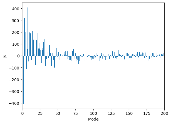
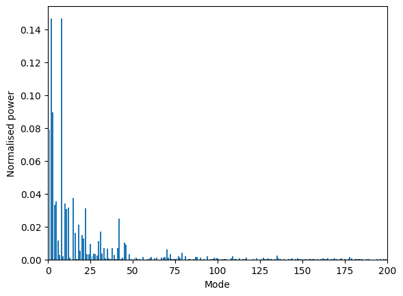
Since eigenmodes represent standing wave patterns, their signs, and thus the signs of \(\beta\) coefficients, are arbitrary. We can equivalently plot the normalised power (\(|\beta|^2/\Sigma|\beta|^2\)) to more clearly display the dominance of lower modes:

norm_power = calc_norm_power(beta)

plt.bar(range(norm_power.shape[0]), norm_power[:, 0])
plt.xlabel('Mode')
plt.xlim(0, solver.n_modes)
plt.ylabel('Normalised power')
plt.show()

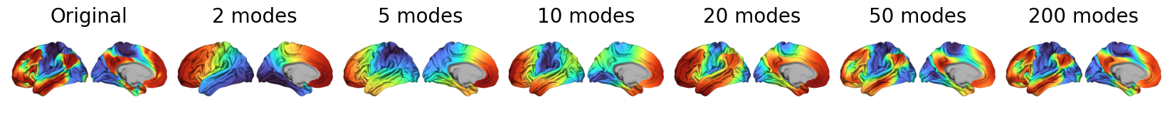
We can reconstruct our map of interest using the first 1-200 modes by calling the reconstruct class method, which will decompose and reconstruct the map, then find the error associated with each reconstruction:

recon, err, beta = solver.reconstruct(masked_map)

# Plot reconstructions next to original map
n_modes_to_plot = [2, 5, 10, 20, 50, 200]
lh_surfpath = files('neuromodes.data') / 'sp-human_tpl-fsLR_den-32k_hemi-L_midthickness.surf.gii'

data = unmask(masked_map, medmask)[:, np.newaxis]  # Original map
for n_modes in n_modes_to_plot:
    recon_map = unmask(recon[:, n_modes - 1, 0], medmask)[:, np.newaxis]
    data = np.concatenate((data, recon_map), axis=1)

with as_file(lh_surfpath) as lh_surfpath:
    plot_surf(lh_surfpath, data, labels=['Original'] + [f'{n} modes' for n in n_modes_to_plot])

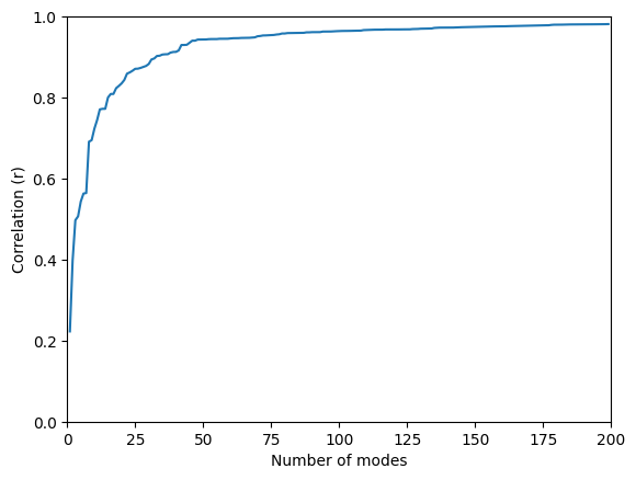
# Plot reconstruction accuracy
plt.plot(1-err[:, 0]) # reports the error (1 - corr) by default
plt.xlabel('Number of modes')
plt.ylabel('Correlation (r)')
plt.xlim(0, solver.n_modes)
plt.ylim(0, 1)
plt.show()